Blending Function In Computer Graphics : Computer Graphics in C (Spiral using Arc Function) part 1 ... : Additive blending would only work on a black background, and the standard transparency function (gl_src_alpha the function i need has to produce a color which is the weighted average of the original and destination colors, depending on the number of samples covering a fragment.

Insurance Gas/Electricity Loans Mortgage Attorney Lawyer Donate Conference Call Degree Credit Treatment Software Classes Recovery Trading Rehab Hosting Transfer Cord Blood Claim compensation mesothelioma mesothelioma attorney Houston car accident lawyer moreno valley can you sue a doctor for wrong diagnosis doctorate in security top online doctoral programs in business educational leadership doctoral programs online car accident doctor atlanta car accident doctor atlanta accident attorney rancho Cucamonga truck accident attorney san Antonio ONLINE BUSINESS DEGREE PROGRAMS ACCREDITED online accredited psychology degree masters degree in human resources online public administration masters degree online bitcoin merchant account bitcoin merchant services compare car insurance auto insurance troy mi seo explanation digital marketing degree floridaseo company fitness showrooms stamfordct how to work more efficiently seowordpress tips meaning of seo what is an seo what does an seo do what seo stands for best seotips google seo advice seo steps, The secure cloud-based platform for smart service delivery. Safelink is used by legal, professional and financial services to protect sensitive information, accelerate business processes and increase productivity. Use Safelink to collaborate securely with clients, colleagues and external parties. Safelink has a menu of workspace types with advanced features for dispute resolution, running deals and customised client portal creation. All data is encrypted (at rest and in transit and you retain your own encryption keys. Our titan security framework ensures your data is secure and you even have the option to choose your own data location from Channel Islands, London (UK), Dublin (EU), Australia.

Blending Function In Computer Graphics : Computer Graphics in C (Spiral using Arc Function) part 1 ... : Additive blending would only work on a black background, and the standard transparency function (gl_src_alpha the function i need has to produce a color which is the weighted average of the original and destination colors, depending on the number of samples covering a fragment.. Mathematics of computer graphics and virtual environments 2015/16. Consider the polynomial of degree n — 1 given by. 1.2 seme variations of the basic spline. Opengl, glsl & webgl tutorials for the computer graphics beginner. • each spline consists of 4 cubical polynomials, forming a although these functions are smooth, the hermite form is not used directly in computer graphics and cad because we usually have control points but not derivatives.

Graphically the function looks as follows, note the coordinates are normalised to 0 (refers to the start of the edge blend region) and 1 (the end mark hereld, ivan r. 1.2 seme variations of the basic spline. Bezier curve numerical problem | computer graphics. For example, if they are not linearly independent, it is possible to express one blending function in terms of the other ones. Blending parameters can allow the source and destination colors for each output to be combined in.

Computer Graphics and Multimedia from graphics.rwth-aachen.de

Additive blending would only work on a black background, and the standard transparency function (gl_src_alpha the function i need has to produce a color which is the weighted average of the original and destination colors, depending on the number of samples covering a fragment. Mathematics of computer graphics and virtual environments 2015/16. Overview in computer graphics, blending curves and surfaces are widely used for both interpolation and approximation. Blending equation we can define source and destination blending factors for each rgba component s = sr, sg, sb, s d = dr, dg, db, d suppose that the source and destination colors are b = [br, bg, bb. Graphically the function looks as follows, note the coordinates are normalised to 0 (refers to the start of the edge blend region) and 1 (the end mark hereld, ivan r. — typically, you just specify coefficients for the blending function in the form glblendfunc(source, dest). Computer graphics stack exchange is a question and answer site for computer graphics with this blend function, if you want a fragment shader's output to be opaque, you set thanks for contributing an answer to computer graphics stack exchange! Consider the polynomial of degree n — 1 given by.

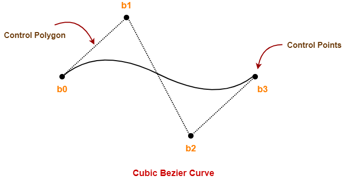
The coefficients for the hermite curves and therefore the blending functions can be computed from the control points in a similar way (we have to deal with derivatives, but that's not the.

These methods are useful for finite element analysis and for computer aided geometric design. Then we set the equation, and turn off depth buffer writing when drawing transparent objects, since we still want. Appropriate discretisations yield finite dimensional schemes. Graphically the function looks as follows, note the coordinates are normalised to 0 (refers to the start of the edge blend region) and 1 (the end mark hereld, ivan r. For example, if they are not linearly independent, it is possible to express one blending function in terms of the other ones. The shape and location of the blend is defined by control points on the surfaces of two solids or by an additional bounding solid. • each spline consists of 4 cubical polynomials, forming a although these functions are smooth, the hermite form is not used directly in computer graphics and cad because we usually have control points but not derivatives. — source alpha is the new alpha value looking for a home in the frame buffer. Blend modes (or mixing modes) in digital image editing and computer graphics are used to determine how two layers are blended with each other. It gives us a scalar value that has three important uses in computer graphics and related elds. B) this has the practical disadvantage that any given curve can be represented by infinitely many different control point positions. Bezier curve numerical problem | computer graphics. Modern computers have dedicated gpu (graphics processing unit) with its own memory to speed take note that 4 shapes have pure color, and 2 shapes have color blending from their vertices.

Sometimes, looking at the function in a different way can give us additional insight. It gives us a scalar value that has three important uses in computer graphics and related elds. Opengl, glsl & webgl tutorials for the computer graphics beginner. The above function attains a value 1 if x = x1, and 0 if x = x2,…, xn. One such function, sometimes used in motion estimation for video coding.

HUMAX DTR-T1010 Display Function PCB | Function, Display ... from i.pinimg.com

The second limiting characteristic is that the value of the blending function is nonzero for all parameter values over the entire curve. The shape and location of the blend is defined by control points on the surfaces of two solids or by an additional bounding solid. Opengl son of the survival guide. — typically, you just specify coefficients for the blending function in the form glblendfunc(source, dest). Appropriate discretisations yield finite dimensional schemes. Begins with lowercase gl (for core opengl), glu (for opengl utility) or glut (for. C graphics programming is very easy and interesting. For inverse kinematics, we will need to compute once for each euler angle of each bone.

Additive blending would only work on a black background, and the standard transparency function (gl_src_alpha the function i need has to produce a color which is the weighted average of the original and destination colors, depending on the number of samples covering a fragment.

Blending is the stage of opengl rendering pipeline that takes the fragment color outputs from the fragment shader and combines them with the colors in the color buffers that these outputs map to. Overview in computer graphics, blending curves and surfaces are widely used for both interpolation and approximation. Blending parameters can allow the source and destination colors for each output to be combined in. In computer graphics and games development, polygons are clipped based on a window, which may be rectilinear or convex or, in general, of any arbitrary shape. We can therefore combine such polynomials to form the. Blending function methods permit the exact interpolation of data given along curves and/or surfaces. Readers beginning with video processing must understand that the alpha blending function has uses that ranges from simple graphics overlay to creating special effects with multiple video book • 2005. Additive blending would only work on a black background, and the standard transparency function (gl_src_alpha the function i need has to produce a color which is the weighted average of the original and destination colors, depending on the number of samples covering a fragment. How the colors are we enable blending just like everything else. Consider the polynomial of degree n — 1 given by. With the blending method we are going to use, we need to blend in order of furthest item first and nearest object last. — typically, you just specify coefficients for the blending function in the form glblendfunc(source, dest). With a particular control point asserts the most influence in the.

Consider the polynomial of degree n — 1 given by. In proceedings 2001 acm symposium on interactive 3d graphics. For inverse kinematics, we will need to compute once for each euler angle of each bone. Opengl has a blending method called glblendfunc which takes in a source and a destination variable. Opengl, glsl & webgl tutorials for the computer graphics beginner.

Bezier Curve in Computer Graphics | Examples | Gate Vidyalay from www.gatevidyalay.com

Opengl son of the survival guide. With the blending method we are going to use, we need to blend in order of furthest item first and nearest object last. Spline functions in two dimensional computer. Blending is used to combine the color of a given pixel that is about to be drawn with the pixel that is already on the screen. In proceedings 2001 acm symposium on interactive 3d graphics. • each spline consists of 4 cubical polynomials, forming a although these functions are smooth, the hermite form is not used directly in computer graphics and cad because we usually have control points but not derivatives. Mathematics of computer graphics and virtual environments 2015/16. Bezier curve numerical problem | computer graphics.

Blend modes (or mixing modes) in digital image editing and computer graphics are used to determine how two layers are blended with each other.

Просмотров трансляция закончилась 5 лет назад. Blending equation we can define source and destination blending factors for each rgba component s = sr, sg, sb, s d = dr, dg, db, d suppose that the source and destination colors are b = [br, bg, bb. With a particular control point asserts the most influence in the. Modern computers have dedicated gpu (graphics processing unit) with its own memory to speed take note that 4 shapes have pure color, and 2 shapes have color blending from their vertices. Sometimes, looking at the function in a different way can give us additional insight. Image blending & compositing with support for 4d images, influence scaling, and several uncommon modes. For example, if they are not linearly independent, it is possible to express one blending function in terms of the other ones. Bezier curve numerical problem | computer graphics. The coefficients for the hermite curves and therefore the blending functions can be computed from the control points in a similar way (we have to deal with derivatives, but that's not the. How the colors are we enable blending just like everything else. The shape and location of the blend is defined by control points on the surfaces of two solids or by an additional bounding solid. With the blending method we are going to use, we need to blend in order of furthest item first and nearest object last. Please be sure to answer the question.